AI - Neural Networks and Deep Learning - Nielsen - Chap 1 Introduction

I came across this book entitled Neural Networks and Deep Learning, by Michael Nielsen, and decided to invest some time in reading it.  I am hoping to reinforce what I have read thus far (for instance in the book AI Crash Course by Haydelin de Ponteves).

The first chapter in this book covers recognition of hand-written digits. This is a pretty cool use case for AI technology, given that everyone's individual handwriting constitutes a font in and of itself, and even then, there is a certain degree of variation every time an individual hand-writes characters. Who uses technology like this? Well, banks for example might use something like this as part of check processing!

I like the fact that this example is optical in nature - and, it could even be inverted in a Generative AI manner to generate new fonts, or new characters in some context or use case!

One of the first things this book covered was Perceptrons - and explained how Perceptrons are essentially binary (1s and 0s) as result output of action functions. He then moves on to explain that binary results are not always in demand or optimal, and that gradient values (shades of gray) between 0 and 1 are often desired or necessary. And this is why we have Sigmoid Neurons. 

This was insightful, because the first book I read (unless I overlooked) never even mentioned the concept of Perceptrons, and jumped right into Sigmoid Neurons.

Nielsen then goes on to explain, briefly, the architecture of Neural Networks and embarks on a practical example using the Handwritten Digits Recognition use case.

One thing that was helpful in this chapter, was the fact that he explains how these hidden layers of a neural network "fit together" by use of a practical example. This helps as far as design and modeling of a Neural Network go.

He goes on to discuss the purpose of using bias along with weights, and then goes into a deeper discussion on gradient descent - and stochastic gradient descent. Stochastic Gradient Descent is critical for reinforcement learning because it minimizes the cost function. Minimizing a cost function does no good though, if you can't "remember" it, so the concept of back propagation is required to instill back into the model, this minimization of cost.

I downloaded the code for his Handwriting Recognition example. I immediately figured out by reading the README.txt file (most people ignore this and waste time learning the harder way) that the code was not written for Python3. Fortunately, someone else had ported the code to Python3 - and this was in another Github repository.  

In running the code from the Python3 repository, I immediately ran into an error with a dependent library called Theano. This error was listed here: Fix for No Section Blas error 

So I was fortunate. This fix worked for me. And we got a successful run! In this example, the accuracy in recognizing handwritten digits was an astounding 99.1%!

This code uses a data sample from MNIST, comprised of 60K samples. The code by default breaks this into a 50/10 training and validation sample.

So now that we know that we can run the code successfully, what might we want to do next on this code, in this chapter, before moving on to the next chapter?

• Experiment with the number of Epochs
  
• Experiment with the Learning Rate
• Experiment with the Mini Batch Size
• Experiment with the number of hidden neurons
  

Here is a table that shows some results from playing with the epochs and mini batch sizes:

test.py

Run 1: Epochs=30, Mini Batch Size=10, Results: 8700/10,000at its peak in epoch 26

Run 2: Epochs=40, Mini Batch Size=10,Results: 9497/10,000 at its peak in epoch 36

Run 3: Epochs=40, Mini Batch Size=20,Results: 9496/10,000 at its peak in epoch 36

So interestingly, the numbers go up each epoch, until a peak is reached, and then the number settles back down for the last 2-3 epochs in these trial runs.  It appears, that the number of epochs is a more important coefficient than the mini batch size. 

Another test with adjusted learning rates could be interesting to run, as this impacts Gradient Descent quite a bit. As Gradient Descent is a Calculus concept for finding the minimum, when learning rates are too low or too high, it impacts the time and ability for the "ball to drop to the bottom" of said low point.

He also, at the very end, mentions the use of more/different algorithms, referencing the Support Vector Machine (SVM).

Artificial Intelligence - LTSM for Financial Modeling - Part II

As Part II of my foray into Stock Portfolio Optimization, I decided to implement Python code that I found in a blog: https://www.datacamp.com/tutorial/lstm-python-stock-market

This blog was written by a Data Scientist, Thuresan Ganegedar . And he spent some time on this. I was super excited after I read the blog, to go in and compile the code and run it myself. The first thing I did, was get myself an API Key so that I could fetch data for a stock symbol.

But - I had issue after issue in running this code. 

First, the code was sufficiently outdated that many libraries, especially Keras, had "moved on" and completely deprecated certain libraries, calls, etc. I spent considerable time picking through the code, doing web searches, and trying to "just get the code to run". 

Second, the code was using hard-coded array values for the number of data points for the stock symbol, and because of this, I ran into null exceptions because the number of data points I had in my stock symbol fetch was over 2K less than the example had. To get around this, I wound up going with 4000 training data points and 600 testing data points. Later, I enhanced the code to dynamically set the training and testing sizes based on how many data points came down in a csv, on a percentage basis.

I also decreased the window size and the batch size as well.

In the end, I was able to produce nice graphs that matched the ones in his blog for the Predictions based on Simple Average and Exponential Moving Average. But these graphs are based on algorithms, not a neural AI network - in other words, they aren't "true AI".

The AI portions of the code did run to completion, but the graphs that came out from implementing the AI, did not look correct. The price predictions were FAR FAR lower than the actuals, as well as the ones from the Simple and Exponential Moving Average graphs.

I may come back and take another look at this, but it was a good exercise, and this exercise made me realize that I need to read and learn more about AI - and what is going on "under the hood".

Artificial Intelligence Book 1 - Using Images in AI - Deep Convolutional Q Learning

I just finished Chapter 12 in my AI Crash Course book, from Hadelin de Ponteves.

Chapter 12 is a short chapter actually. It explains, in a refreshing and surprising simple way, the concept of Convolutional Q Learning which pertains to how image recognition/translation is fed into a Deep Q Neural Network (from prior chapters in the book).

The chapter covers four steps:

1. Convolution - applying feature detectors to an image
   
2. Max Pooling - simplifying the data
   
3. Flattening - taking all of the results of #1 and #2 and putting them into a one-dimensional array
   
4. Full Connection - feeding the one-dimensional array as Inputs into the Deep Q Learning model
   

I probably don't need to go over all of these details in this blog as that would be redundant. 

If you have some exposure to Computing and are familiar with Bitmaps, I think this process has shares some conceptual similarity to Bitmaps. 

For example, in Step 1 - Convolution - you are essentially sliding a feature detector or "filter" (e.g. 3x3 in the book) over an image - starting on Row 1, and sliding it left to right one one column at a time before dropping down to Row 2 and repeating that process. On each slide interval, you are employing a mapping process of multiplying each square of the image (again using a 3z3 area in the book) to the corresponding value of the map. Each individual iteration of this process creates a single Feature Map. 

In sliding this 3x3 map across, you can only go 5 times to the right before you run out of real estate. Then you drop down - and you can only drop down 5 times until you run out of real estate in that direction. So if I am correct in my interpretation about how this works, you would get 5 x 5 = 25 Feature Maps with a 7x7 image and a 3x3 filter.

Pooling is actually similar to the process of filtering to a feature map. The aim of it is to reduce the size and complexity of all of those feature maps. The sliding process is the main difference; instead of going one column / row on each slide, you are sliding (using a 2x2 in the book) over the entire area of the pool size.

Once you get all of the pools, these are flattened out into a single dimensional array, and fed into the Inputs of the standard Q Learning model, with the outputs pertaining to image recognition.

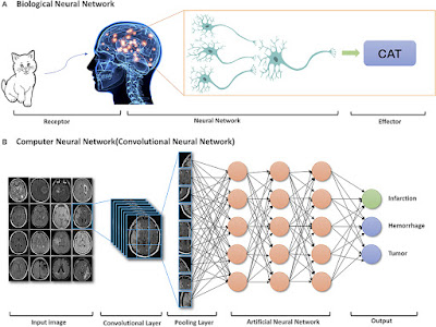
This diagram shows how all of this is done, with a nice comparison between Biological image recognition, with this AI image recognition process.

Image Recognition - Biological vs AI

Source: frontiersin.org

Now in Chapter 12 of the book, the process represents what we see above. There is just a single Convolutional Layer and Pooling Layer before the AI Neural Network (hidden layers) are engaged. 

Chapter 12 does not cover the fact that the Convolutional Layer is an iterative process that includes Convolution followed by Sub-Sampling in an iterative fashion. 

This diagram below represents this.

In the next chapter, there is a code sample, so I will be able to see whether it includes this sub-sampling process or not.

Artificial Intelligence Book 1 - Crash Course in AI - Deep Q Learning

 I read about Q Learning, and was feeling somewhat proud of myself for sticking my toe into the water.

Then I read about Deep Q Learning - in this same book - and it was as if someone took an ice bath and dumped it over my head. I went into the tunnel - advancing through chapters 9,10 and 11, only to come out the other end confused ("what did I just read?").  

The coding examples were interesting enough that I kept pushing forward, but a lot of what is in the code is masked by the fact that the math and formulas were hidden away in libraries like Keras.  So while I thought the examples were cool and I had a grasp of the problems they were attempting to solve, I still came out at the end with confusion and question marks in my head.

Q Learning vs Deep Q Learning

 In Chapter 9, which covers Deep Q-Learning, things start to get very complex very fast. So what is the difference between Q Learning (introduced in Chapter 7-8), and Deep Q Learning?

• More complex problems in Deep Q Learning - with more variables
• The approach to solving a more complex problem
  

With regards to the approach to solving problems, the book gets into a good discussion - worth mentioning here - about the difference between ArgMax and SoftMax.

Argmax vs Softmax

In Q Learning, the 'name of the game' was to find (and use) the highest Q Value. This is referred to as "Exploitive" and is known as the ArgMax method of Reinforcement Learning.  

In Deep Q Learning, probability distributions across several variables are being continually updated during the training of the model. You have a set of (input) variables, with specific weights, but as you take random samples and compare the predicated value to the actual value, the weights are updated according to the new realities (results).  This process is referred to as Explorative (in nature) and is named the SoftMax method.

Chapter 9 starts you off simple(r). With a Real Estate example of predicting home prices. Seems sensible enough, since we can all think of input variables that help drive the price of a home.  The focus here is on trying to show the process, which is broken down into the following steps:

1. Uploading the Data Set (actual home prices)
2. Building the Neural Network
3. Training the Neural Network
4. Displaying the Results

From here, the book advances into Deep Learning Theory. The idea borrows from the human brain, which is connected by Synapses that send signals. This is the fundamental concept behind Deep Q Learning because it starts with a certain number of "Layers". There are a minimum of three layers that are as follows:

1. Input Layer - consists of Input Values, and each of these gets weights that are continually adjusted
   
2. Hidden Layer(s) - these "neurons" are also continually adjusted
   
3. Output Layer - this layer compares predicted values to actual values and computes Loss Error.
   

The loss error gets back-propagated through the layers, re-adjusting the weights continually, using a concept called Gradient Descent (which requires at least a basic understanding of Calculus). The book covers three types of Gradient Descent (Batch, Stochastic and Mini-Batch).

The book mentions Activation Functions that take weighted input values, and return an output value. The book mentions three of these, which sound intimidating, but if you are familiar with Electronics and/or Trigonometry, these names actually make some sense:

• Sigmoid Activation Function - a logarithmic curve denoting a move from state value (no lower than) 0 to (no higher than) 1.
• Rectifier Activation Function - a linear but angular approach from state 0 to state 1
• Threshold Activation Function - An abrupt binary state transition from 0 to 1. This is much like flipping a switch into an on/off state.

Now from here (Chapter 9), the book goes into Chapter 10 - Self Driving Car - which an implementation of Chapter 9 - and quite fun to do. Then it dives into Chapter 11, which uses the example taken from Google's DeepMind project that optimizes server temperature with a simulation.

Chapter 11 in particular really drives home the process by showing how you can optimize or minimize costs.

1. Building the Environment
2. Building the Brain - using DropOut vs NoDropOut techniques
   
3. Implementation (of the Deep Learning Algorithm)
4. Training the AI - using either Early Stopping or No Early Stopping
5. Testing the AI
   

Seeing is believing, and when you see this code run and start to view the results, I have to admit it is pretty darn cool.

It also takes a LONG time to run. I had to shorten the epochs from 100 to 25 to keep the job from getting killed (I am not sure what exactly was killing it). Running for 100 epochs was taking my laptop HOURS to finish (2-3 hours). But at the end of each Epoch, almost always the energy savings from the AI was superior to the energy savings of not using the AI (which in this case is modeled by the server's mainboard temperature controller).

There's so much more to discuss. But I think I have hit the highlights here.