Artificial Intelligence Book 1 - Using Images in AI - Deep Convolutional Q Learning

I just finished Chapter 12 in my AI Crash Course book, from Hadelin de Ponteves.

Chapter 12 is a short chapter actually. It explains, in a refreshing and surprising simple way, the concept of Convolutional Q Learning which pertains to how image recognition/translation is fed into a Deep Q Neural Network (from prior chapters in the book).

The chapter covers four steps:

1. Convolution - applying feature detectors to an image
   
2. Max Pooling - simplifying the data
   
3. Flattening - taking all of the results of #1 and #2 and putting them into a one-dimensional array
   
4. Full Connection - feeding the one-dimensional array as Inputs into the Deep Q Learning model
   

I probably don't need to go over all of these details in this blog as that would be redundant. 

If you have some exposure to Computing and are familiar with Bitmaps, I think this process has shares some conceptual similarity to Bitmaps. 

For example, in Step 1 - Convolution - you are essentially sliding a feature detector or "filter" (e.g. 3x3 in the book) over an image - starting on Row 1, and sliding it left to right one one column at a time before dropping down to Row 2 and repeating that process. On each slide interval, you are employing a mapping process of multiplying each square of the image (again using a 3z3 area in the book) to the corresponding value of the map. Each individual iteration of this process creates a single Feature Map. 

In sliding this 3x3 map across, you can only go 5 times to the right before you run out of real estate. Then you drop down - and you can only drop down 5 times until you run out of real estate in that direction. So if I am correct in my interpretation about how this works, you would get 5 x 5 = 25 Feature Maps with a 7x7 image and a 3x3 filter.

Pooling is actually similar to the process of filtering to a feature map. The aim of it is to reduce the size and complexity of all of those feature maps. The sliding process is the main difference; instead of going one column / row on each slide, you are sliding (using a 2x2 in the book) over the entire area of the pool size.

Once you get all of the pools, these are flattened out into a single dimensional array, and fed into the Inputs of the standard Q Learning model, with the outputs pertaining to image recognition.

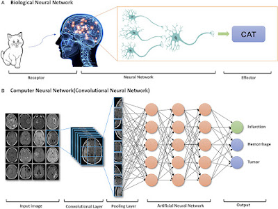
This diagram shows how all of this is done, with a nice comparison between Biological image recognition, with this AI image recognition process.

Image Recognition - Biological vs AI

Source: frontiersin.org

Now in Chapter 12 of the book, the process represents what we see above. There is just a single Convolutional Layer and Pooling Layer before the AI Neural Network (hidden layers) are engaged. 

Chapter 12 does not cover the fact that the Convolutional Layer is an iterative process that includes Convolution followed by Sub-Sampling in an iterative fashion. 

This diagram below represents this.

In the next chapter, there is a code sample, so I will be able to see whether it includes this sub-sampling process or not.